Optimal Fitness Machine Allocation using OR-Tools
Posted March 7, 2026 by Victor Sonck ‐ 12 min read
In Belgium, there’s this thing called “rugschool”, which translates directly to “backschool”. “back” as in your anatomical spine. It’s a combination of theory lessons on anatomy, pain, psychology, ergonomics etc as well as 4 machines that train up your core muscles and 1 more optional one for your neck muscles.
As it happens, I’m a patient in “backschool” and there’s something that’s bothering me about the machines: the patient to machine allocation.
Patients just naively take any machine that’s free and end up waiting around for equipment to free up for a long time and that bothers me.
Yes, I realise I’m a nerd that looks at fitness equipment and the first thing that comes to mind is that the patient allocation algorithm could be improved 🤷
The patients and the machines
Patients come in around every hour, each of them has a unique training schedule on the machines. Some patients take 9 sets of 20 reps on a machine while others take only 5 sets of 10 on the same machine. The existing software of the machines knows this upfront though, so this info could be taken into account by an allocation optimiser.
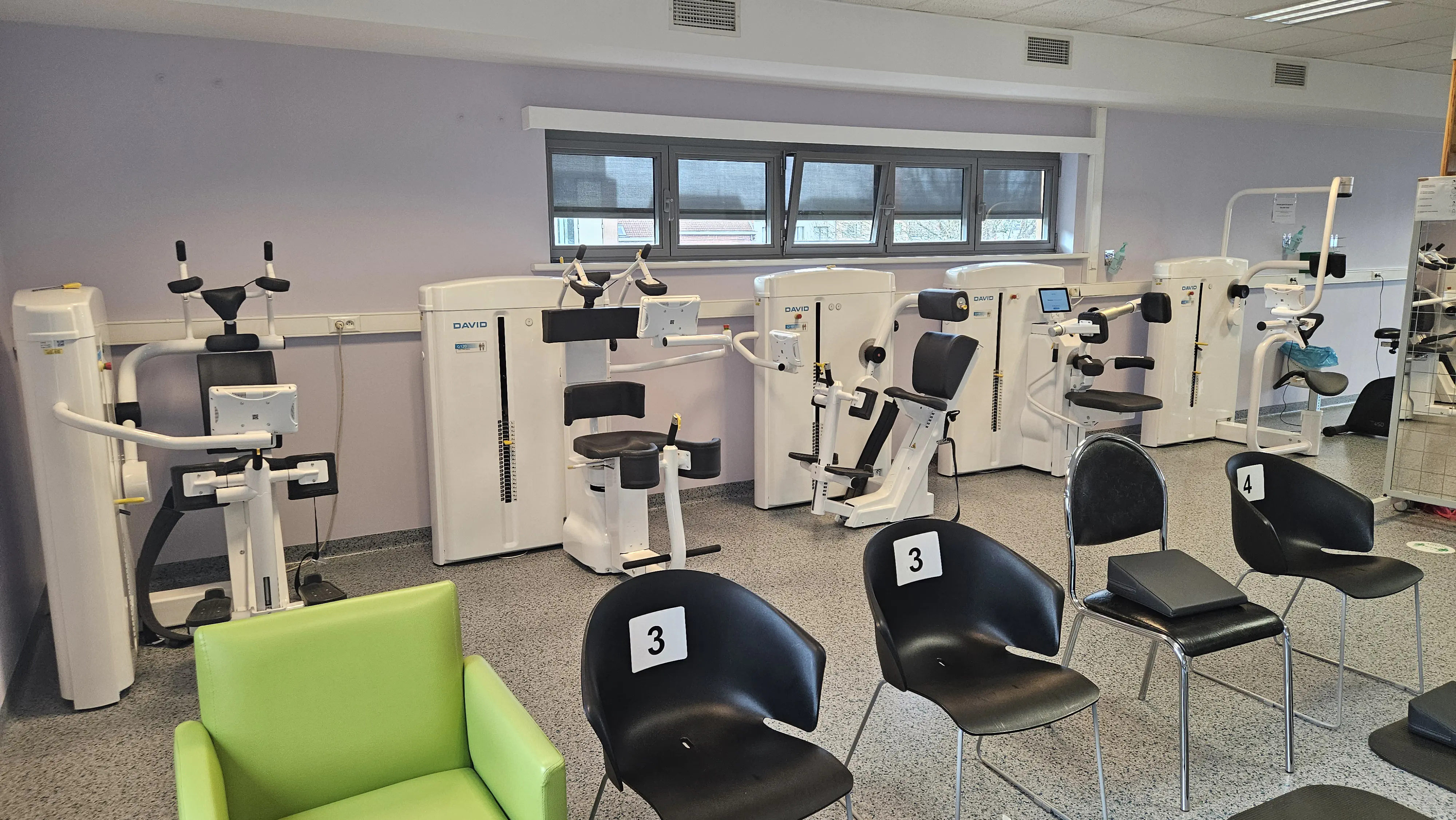
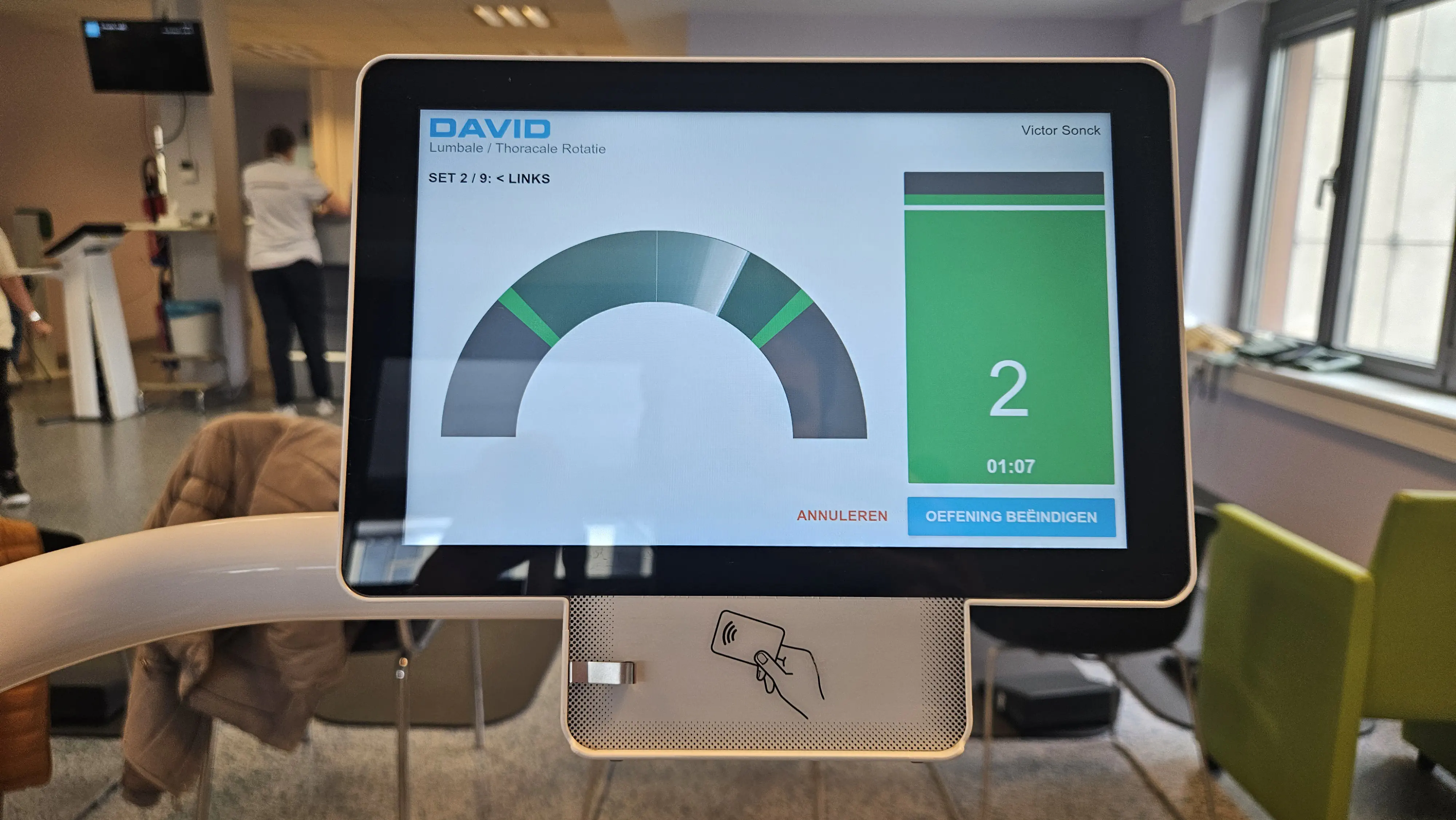
The machines are from the brand “David” and are very fancy. I’ve heard from a friend they can cost up to 25k per machine. They adjust their seat height and other measurements when you tap your personal card on it, they each have a screen showing you live how to do your exercise and they keep track of both your schedule and your performance over time.
There’s machines 1 and 3 for straight belly and back muscles, then machines 2 and 4 for side belly and back. These last ones have to train left as well as right sides, so they take longer. I’ll ignore the optional neck machine, because it simply doesn’t apply to me.
Simulating backschool
Some patients are too early, others too late. I distributed the arrival times around every hour as a normal distribution with a standard deviation of 5 minutes. So 99.7% of the arrivals will be within 15 minutes of the hour.
The amount of people arriving each hour is a parameter I wanted to be able to play with. In real life this varies from 2 or 3 to maybe 6 on some days.
Then I randomly generated a training schedule for each patient. Machine 1 and 3 have duration between 5 and 10 minutes. Machine 2 and 4 between 10 and 15 minutes. These estimates are based on my anecdotal evidence from the real training room. Each arriving person gets a training schedule assigned upfront, which mimics the real situation where the system knows (approximately) how long each exercise of each patient should take.
So now we have a timeline, people arriving at random times on that timeline. We can simulate their personalised time spent on each machine and track their potential time waiting for a machine to free up.
Because of the magic of LLMs, I vibecoded up a debug interface that visualises the patient allocations, because it always helps to have clear visual examples.

The naive approach
In real life, I have been observing how people decide what machine to pick. In the vast majority of cases, they just pick the machine that’s free at that moment and if there are multiple, they pick basically randomly. We’ll call this the naive strategy.
We can now code this strategy up into code and run some simulations, here are the results:
====================================================================================================
GRID SEARCH: Naive Strategy Baseline
Hours: 1-8, Arrivals/hr: 1-7, Runs per cell: 10
====================================================================================================

Hours\Arr/h │      1       │      2       │      3       │      4       │      5       │      6       │      7       │
────────────┼──────────────┼──────────────┼──────────────┼──────────────┼──────────────┼──────────────┼──────────────┤
     1h     │   0.0 min    │   0.6 min    │   2.5 min    │   7.8 min    │   13.0 min   │   17.9 min   │   22.3 min   │
     2h     │   0.0 min    │   0.3 min    │   2.5 min    │   7.7 min    │   15.2 min   │   25.2 min   │   35.4 min   │
     3h     │   0.0 min    │   0.4 min    │   2.0 min    │   6.8 min    │   16.8 min   │   30.6 min   │   49.1 min   │
     4h     │   0.0 min    │   0.9 min    │   2.3 min    │   7.4 min    │   17.2 min   │   38.6 min   │   63.6 min   │
     5h     │   0.0 min    │   0.7 min    │   2.7 min    │   7.1 min    │   20.7 min   │   46.7 min   │   75.6 min   │
     6h     │   0.0 min    │   0.5 min    │   2.8 min    │   7.4 min    │   20.2 min   │   53.5 min   │   91.7 min   │
     7h     │   0.0 min    │   0.4 min    │   2.3 min    │   7.6 min    │   20.2 min   │   61.0 min   │  107.1 min   │
     8h     │   0.0 min    │   0.5 min    │   2.6 min    │   7.5 min    │   21.0 min   │   68.6 min   │  116.3 min   │
====================================================================================================
Legend: Average wait time per person (minutes)

----------------------------------------------------------------------------------------------------
SUMMARY STATISTICS
----------------------------------------------------------------------------------------------------
  Min avg wait time: 0.0 min/person
  Max avg wait time: 116.3 min/person
  Overall avg wait time: 20.2 min/person
====================================================================================================
The rows are the amount of hours we simulated. From a single hour to a full day. The columns are the amount of patients coming in per hour.
Logically, the 1 patient per hour scenario has no waiting time. But starting already from 2 patients per hour, we already see waiting time starting to show up! It’s less than a minute per person on average, but still, 2 people should be easily manageable for 4 machines, yet the naive strategy fucks things up very quickly.
The scenario with 5 people per hour ramps up average waiting time per person to 15-20 minutes and the 6 people scenario 20-70 minutes. My real life experiences have been that the load varies between 2 and 6 throughout the day and on busy days I get about 20 to 30 minutes of waiting time. That seems to fit the simulated data quite well.
Solving this with OR-tools
There are several ways this naive strategy can be optimised.
Better free machine choices
For one, if there are 2 or more free machines, we could pick the next machine based on what machines the other patients still need to do.
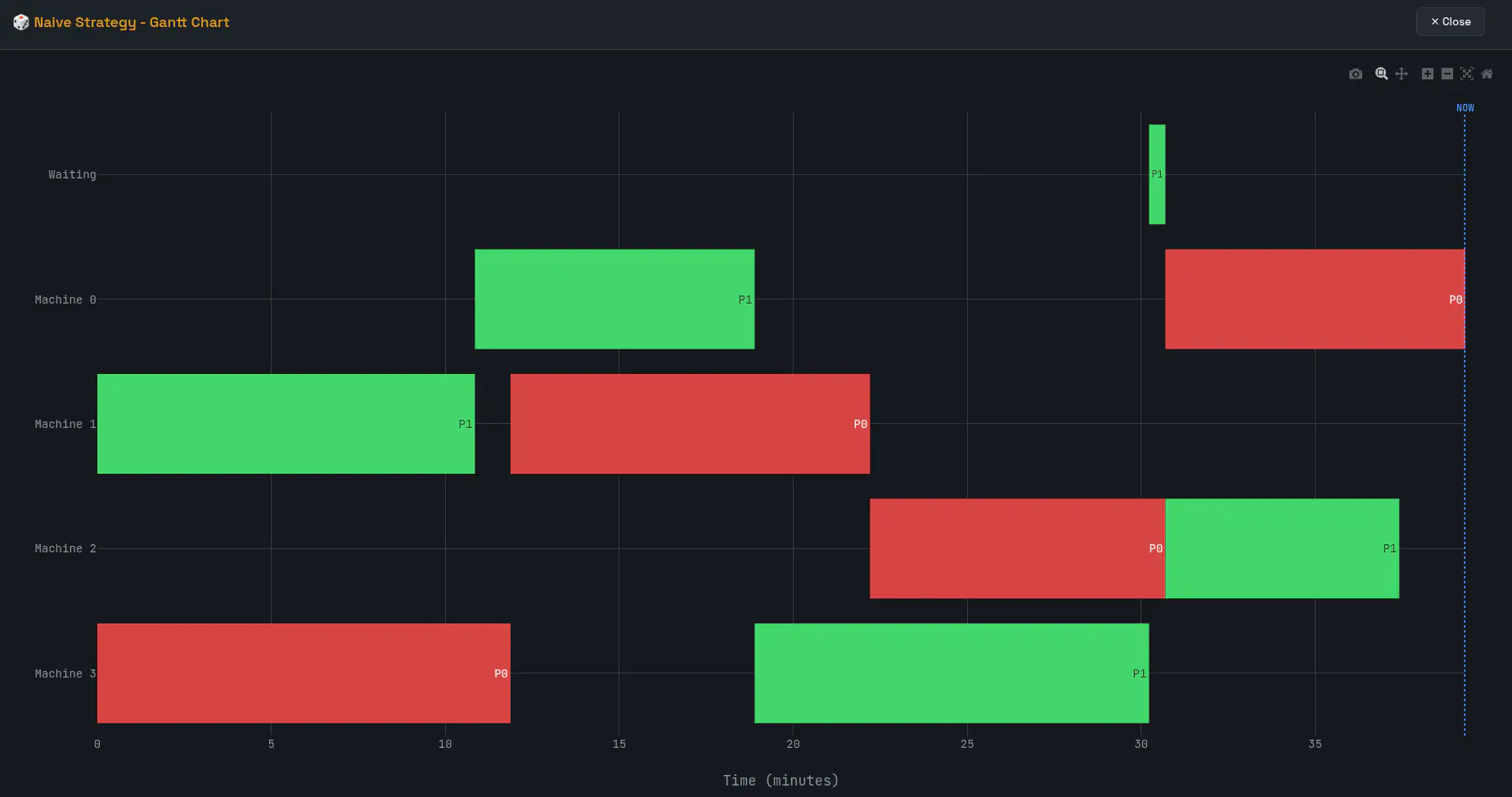
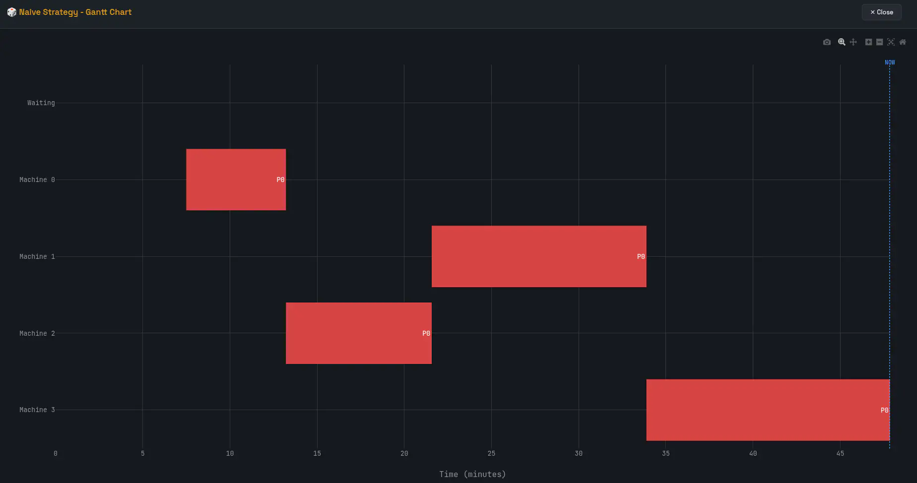
For example here: The naive strategy had Patient 0 (red) choose from 2 free machines at around 23 minutes in. They just happened to pick the one machine (machine 2) that P1 (green) still had to do as their last one. So now P1 (green) has to wait for P0 (red) to finish, for no other reason than bad scheduling. If P0 (red) would have chosen Machine 0 instead, Machine 2 would have been free for P1 (green) when they needed it.
The waiting time here is only half a minute, but it is a simple example and it’s not hard to see how waiting time could be much higher.
Strategic waiting
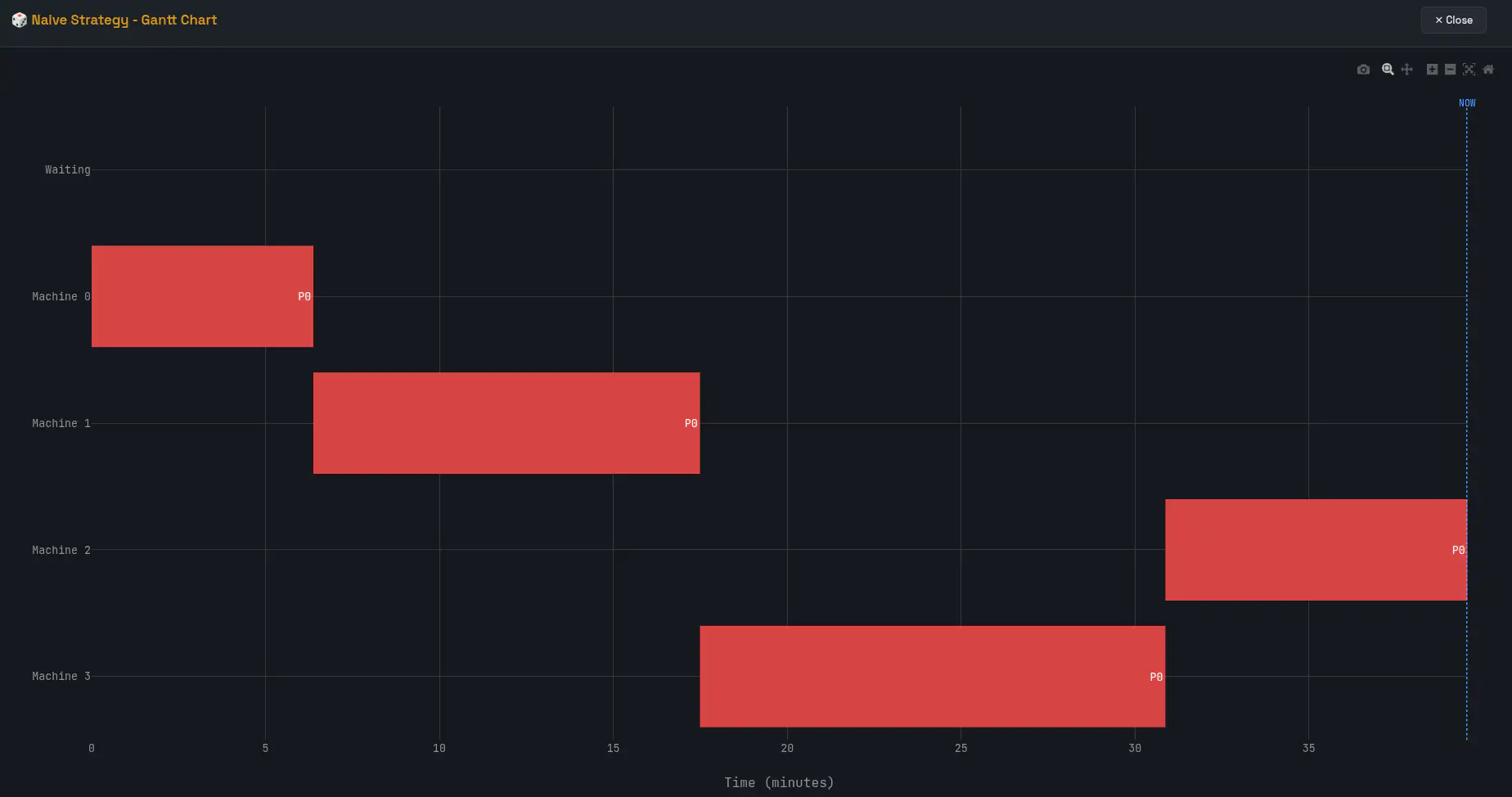
Another approach is what I call strategic waiting. It’s when a single machine is free and instead of taking it, a person can wait a small amount of time for another person to finish their machine first.
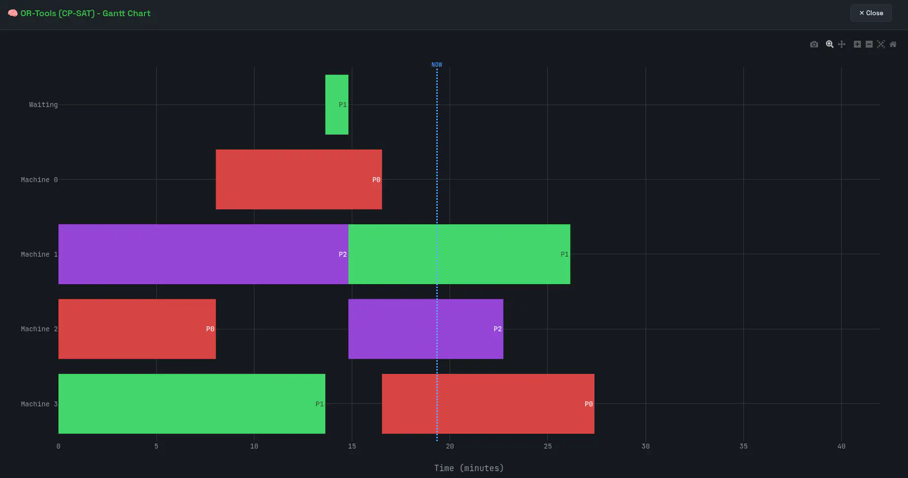
When P1 (green) was done with machine 3, they could have gone straight to machine 2, which was free at that time. Instead, they waited for P2 (purple) to finish, taking machine 1 as soon as they were done, leaving machines 2 and 3 open for P0 (red) and P2 (purple). This then led to a better order down the line.
Google OR-tools
OR-tools is amazing. At ML6, I tried it for the first time to solve a taxi routing problem. It’s not as easy or intuitive to use as naive code, but if you manage to get your problem formulated as an OR tools optimisation problem, it can potentially give you an fully optimal solution in seconds, and will give its best guess with a fixed deadline otherwise, e.g. best you can do in 5 seconds.
In OR-tools’ eyes, this is a classic constrain programming problem. A frequently used example of this type of problem is called the job shop problem.
The OR-Tools docs define this as:
Each job consists of a sequence of tasks, which must be performed in a given order, and each task must be processed on a specific machine. For example, the job could be the manufacture of a single consumer item, such as an automobile. The problem is to schedule the tasks on the machines so as to minimize the
lengthof the schedule—the time it takes for all the jobs to be completed.
There are several constraints for the job shop problem:
• No task for a job can be started until the previous task for that job is completed. • A machine can only work on one task at a time. • A task, once started, must run to completion.
So our little fitness machines can be seen as a factory, only the order in which machines are used does not matter in our case, meaning the first constraint from above here doesn’t apply. We don’t actually have the precedence constraints from the classic job shop problem.
We do have no overlap constraints since one machine can only service one human and one human can only use one machine at a time.
We are also not optimising on minimum time to completion of the last job (which would essentially mean optimal machine efficiency), but instead we want to optimise for minimal patient waiting time, because I don’t like to wait around.
And that’s basically all we need to do!
At any point in time, we can define the start and end intervals of the exercises of the people currently in the system as well as the planned arrivals of any people still coming. Then we add the no overlap constraints and ask the solver to optimise for minimal waiting time. This is called rolling-horizon optimisation and it sounds really cool.
The solver will return an optimal assignment given the current state of the system without ever needing any info that it would not have access to in real life at that point in time (so we’re not looking forward in time!)
Results
====================================================================================================
GRID SEARCH: Naive vs OR-Tools Online
Hours: 1-8, Arrivals/hr: 1-7, Runs per cell: 10
====================================================================================================

Hours\Arr/h │     1      │     2      │     3      │     4      │     5      │     6      │     7      │
────────────┼────────────┼────────────┼────────────┼────────────┼────────────┼────────────┼────────────┤
     1h     │    0.0     │    0.0     │    0.3     │    4.0     │    9.2     │   14.4     │   19.9     │
     2h     │    0.0     │    0.0     │    0.2     │    3.6     │   11.2     │   21.1     │   32.6     │
     3h     │    0.0     │    0.0     │    0.3     │    3.6     │   12.1     │   27.8     │   46.0     │
     4h     │    0.0     │    0.0     │    0.2     │    3.2     │   13.5     │   35.2     │   60.5     │
     5h     │    0.0     │    0.0     │    0.2     │    3.3     │   16.0     │   43.9     │   71.9     │
     6h     │    0.0     │    0.0     │    0.2     │    3.3     │   16.0     │   50.3     │   87.4     │
     7h     │    0.0     │    0.0     │    0.2     │    3.4     │   16.5     │   57.6     │  103.3     │
     8h     │    0.0     │    0.0     │    0.2     │    3.3     │   17.6     │   65.3     │  112.5     │

Legend: ortools average wait time (min/person)

====================================================================================================

Hours\Arr/h │     1      │     2      │     3      │     4      │     5      │     6      │     7      │
────────────┼────────────┼────────────┼────────────┼────────────┼────────────┼────────────┼────────────┤
     1h     │    +0.0%   │   +98.0%   │   +88.2%   │   +48.3%   │   +29.4%   │   +19.5%   │   +11.0%   │
     2h     │    +0.0%   │   +89.4%   │   +93.2%   │   +53.0%   │   +26.0%   │   +16.0%   │    +7.9%   │
     3h     │    +0.0%   │   +95.8%   │   +86.2%   │   +46.8%   │   +28.2%   │    +9.4%   │    +6.5%   │
     4h     │    +0.0%   │   +96.1%   │   +91.4%   │   +56.8%   │   +21.7%   │    +8.7%   │    +5.0%   │
     5h     │    +0.0%   │   +98.1%   │   +91.3%   │   +53.1%   │   +22.6%   │    +6.0%   │    +4.9%   │
     6h     │    +0.0%   │   +93.2%   │   +92.1%   │   +55.9%   │   +21.0%   │    +6.0%   │    +4.7%   │
     7h     │    +0.0%   │   +91.6%   │   +90.1%   │   +55.0%   │   +18.3%   │    +5.6%   │    +3.6%   │
     8h     │    +0.0%   │   +94.6%   │   +91.2%   │   +55.4%   │   +16.0%   │    +4.8%   │    +3.3%   │
====================================================================================================
Legend: % improvement (positive = ortools better)

====================================================================================================

Hours\Arr/h │     1      │     2      │     3      │     4      │     5      │     6      │     7      │
────────────┼────────────┼────────────┼────────────┼────────────┼────────────┼────────────┼────────────┤
     1h     │    0.0     │    0.6     │    2.2     │    3.8     │    3.8     │    3.5     │    2.5     │
     2h     │    0.0     │    0.3     │    2.4     │    4.1     │    4.0     │    4.0     │    2.8     │
     3h     │    0.0     │    0.4     │    1.8     │    3.2     │    4.7     │    2.9     │    3.2     │
     4h     │    0.0     │    0.9     │    2.1     │    4.2     │    3.7     │    3.3     │    3.2     │
     5h     │    0.0     │    0.7     │    2.4     │    3.8     │    4.7     │    2.8     │    3.7     │
     6h     │    0.0     │    0.4     │    2.5     │    4.2     │    4.2     │    3.2     │    4.3     │
     7h     │    0.0     │    0.4     │    2.1     │    4.2     │    3.7     │    3.4     │    3.8     │
     8h     │    0.0     │    0.5     │    2.4     │    4.1     │    3.4     │    3.3     │    3.9     │

Legend: Average time saved per person ortools vs naive (min)

====================================================================================================

Hours\Arr/h │     1      │     2      │     3      │     4      │     5      │     6      │     7      │
────────────┼────────────┼────────────┼────────────┼────────────┼────────────┼────────────┼────────────┤
     1h     │    0.0     │    1.2     │    6.6     │   15.0     │   19.2     │   20.9     │   17.2     │
     2h     │    0.0     │    1.2     │   14.2     │   32.8     │   39.5     │   48.3     │   39.4     │
     3h     │    0.0     │    2.5     │   15.8     │   38.3     │   71.2     │   52.1     │   66.9     │
     4h     │    0.0     │    7.1     │   25.5     │   67.4     │   74.9     │   80.3     │   88.3     │
     5h     │    0.0     │    6.4     │   36.4     │   75.4     │  117.1     │   84.0     │  130.1     │
     6h     │    0.0     │    5.2     │   45.7     │   99.9     │  127.3     │  116.4     │  179.4     │
     7h     │    0.0     │    4.9     │   44.2     │  117.0     │  128.9     │  144.0     │  186.6     │
     8h     │    0.0     │    8.0     │   57.3     │  132.4     │  134.7     │  157.3     │  216.2     │

Legend: Total human time saved per day ortools vs naive (min)
Conclusion
The results speak for themselves. Between 2 and 5 arrivals per hour, which covers the typical backschool load, we can save significant amounts of time. At 2 arrivals per hour, the optimisation nearly eliminates waiting altogether (90%+ improvement). At 4 arrivals, we’re still cutting wait times roughly in half. Even at 5 arrivals, we’re shaving off 20–30% of the time people would otherwise spend standing around.
The average savings per person might look modest: a few minutes here and there. But averages hide the full picture. Some people will have to wait much longer than others when the naive strategy sends everyone to the same machines at the wrong times. That variance is exactly what the optimiser smooths out. It’s not just about the average, it’s about not leaving anyone stuck waiting 20 minutes while three machines sit idle.
Scale it up over a full day and the numbers add up. On a busy 8-hour day with 6 or 7 people per hour, we’re talking about 2 hours or more of cumulative human time saved. That’s 2 hours of human time we could have spent elsewhere.
Next to time saved, I wouldn’t be surprised if a hospital would want this as well. Those 2 hours could end up equating to 2 more patients you can take on per day. David, if you ever read this, hit me up!